Mathematical expectation of a random variable. Mathematical expectation of a continuous random variable Linearity of mathematical expectation

Probability theory is a special branch of mathematics that is studied only by students of higher educational institutions. Do you like calculations and formulas? You are not afraid of the prospects of getting acquainted with the normal distribution, ensemble entropy, mathematical expectation and discrete dispersion random variable? Then this subject will be very interesting to you. Let's take a look at a few of the most important basic concepts this branch of science.

Let's remember the basics

Even if you remember the simplest concepts of probability theory, do not neglect the first paragraphs of the article. The point is that without a clear understanding of the basics, you will not be able to work with the formulas discussed below.

So, some random event occurs, some experiment. As a result of the actions we take, we can get several outcomes - some of them occur more often, others less often. The probability of an event is the ratio of the number of actually obtained outcomes of one type to total number possible. Only knowing the classical definition of this concept can you begin to study the mathematical expectation and dispersion of continuous random variables.

Average

Back in school, during math lessons, you started working with the arithmetic mean. This concept is widely used in probability theory, and therefore cannot be ignored. The main thing for us is this moment is that we will encounter it in the formulas for the mathematical expectation and dispersion of a random variable.

We have a sequence of numbers and want to find the arithmetic mean. All that is required of us is to sum up everything available and divide by the number of elements in the sequence. Let us have numbers from 1 to 9. The sum of the elements will be equal to 45, and we will divide this value by 9. Answer: - 5.

Dispersion

Speaking scientific language, dispersion is the average square of deviations of the obtained characteristic values ​​from the arithmetic mean. It is denoted by one capital Latin letter D. What is needed to calculate it? For each element of the sequence, we calculate the difference between the existing number and the arithmetic mean and square it. There will be exactly as many values ​​as there can be outcomes for the event we are considering. Next, we sum up everything received and divide by the number of elements in the sequence. If we have five possible outcomes, then divide by five.

Dispersion also has properties that need to be remembered in order to be used when solving problems. For example, when increasing a random variable by X times, the variance increases by X squared times (i.e. X*X). It is never less than zero and does not depend on shifting values ​​up or down by equal amounts. Additionally, for independent trials, the variance of the sum is equal to the sum of the variances.

Now we definitely need to consider examples of the variance of a discrete random variable and the mathematical expectation.

Let's say we ran 21 experiments and got 7 different outcomes. We observed each of them 1, 2, 2, 3, 4, 4 and 5 times, respectively. What will the variance be equal to?

First, let's calculate the arithmetic mean: the sum of the elements, of course, is 21. Divide it by 7, getting 3. Now subtract 3 from each number in the original sequence, square each value, and add the results together. The result is 12. Now all we have to do is divide the number by the number of elements, and, it would seem, that’s all. But there's a catch! Let's discuss it.

Dependence on the number of experiments

It turns out that when calculating variance, the denominator can contain one of two numbers: either N or N-1. Here N is the number of experiments performed or the number of elements in the sequence (which is essentially the same thing). What does this depend on?

If the number of tests is measured in hundreds, then we must put N in the denominator. If in units, then N-1. Scientists decided to draw the border quite symbolically: today it passes through the number 30. If we conducted less than 30 experiments, then we will divide the amount by N-1, and if more, then by N.

Task

Let's return to our example of solving the problem of variance and mathematical expectation. We got an intermediate number 12, which needed to be divided by N or N-1. Since we conducted 21 experiments, which is less than 30, we will choose the second option. So the answer is: the variance is 12 / 2 = 2.

Expected value

Let's move on to the second concept, which we must consider in this article. Expected value is the result of adding all possible outcomes multiplied by the corresponding probabilities. It is important to understand that the obtained value, as well as the result of calculating the variance, is obtained only once for the entire problem, no matter how many outcomes are considered in it.

The formula for mathematical expectation is quite simple: we take the outcome, multiply it by its probability, add the same for the second, third result, etc. Everything related to this concept is not difficult to calculate. For example, the sum of the expected values ​​is equal to the expected value of the sum. The same is true for the work. Not every quantity in probability theory allows you to perform such simple operations. Let's take the problem and calculate the meaning of two concepts we have studied at once. Besides, we were distracted by theory - it's time to practice.

One more example

We ran 50 trials and got 10 types of outcomes - numbers from 0 to 9 - appearing in different percentages. These are, respectively: 2%, 10%, 4%, 14%, 2%,18%, 6%, 16%, 10%, 18%. Recall that to obtain probabilities, you need to divide the percentage values ​​by 100. Thus, we get 0.02; 0.1, etc. Let us present an example of solving the problem for the variance of a random variable and the mathematical expectation.

We calculate the arithmetic mean using the formula that we remember from junior school: 50/10 = 5.

Now let’s convert the probabilities into the number of outcomes “in pieces” to make it easier to count. We get 1, 5, 2, 7, 1, 9, 3, 8, 5 and 9. From each value obtained, we subtract the arithmetic mean, after which we square each of the results obtained. See how to do this using the first element as an example: 1 - 5 = (-4). Next: (-4) * (-4) = 16. For other values, do these operations yourself. If you did everything correctly, then after adding them all up you will get 90.

Let's continue calculating the variance and expected value by dividing 90 by N. Why do we choose N rather than N-1? Correct, because the number of experiments performed exceeds 30. So: 90/10 = 9. We got the variance. If you get a different number, don't despair. Most likely, you made a simple mistake in the calculations. Double-check what you wrote, and everything will probably fall into place.

Finally, remember the formula for mathematical expectation. We will not give all the calculations, we will only write an answer that you can check with after completing all the required procedures. The expected value will be 5.48. Let us only recall how to carry out operations, using the first elements as an example: 0*0.02 + 1*0.1... and so on. As you can see, we simply multiply the outcome value by its probability.

Deviation

Another concept closely related to dispersion and mathematical expectation is standard deviation. It is designated either with Latin letters sd, or Greek lowercase "sigma". This concept shows how much on average the values ​​deviate from the central feature. To find its value, you need to calculate Square root from dispersion.

If you plot a normal distribution graph and want to see the squared deviation directly on it, this can be done in several stages. Take half of the image to the left or right of the mode (central value), draw a perpendicular to the horizontal axis so that the areas of the resulting figures are equal. The size of the segment between the middle of the distribution and the resulting projection onto the horizontal axis will represent the standard deviation.

Software

As can be seen from the descriptions of the formulas and the examples presented, calculating variance and mathematical expectation is not the simplest procedure from an arithmetic point of view. In order not to waste time, it makes sense to use the program used in higher education educational institutions- it's called "R". It has functions that allow you to calculate values ​​for many concepts from statistics and probability theory.

For example, you specify a vector of values. This is done as follows: vector<-c(1,5,2…). Теперь, когда вам потребуется посчитать какие-либо значения для этого вектора, вы пишете функцию и задаете его в качестве аргумента. Для нахождения дисперсии вам нужно будет использовать функцию var. Пример её использования: var(vector). Далее вы просто нажимаете «ввод» и получаете результат.

Finally

Dispersion and mathematical expectation are without which it is difficult to calculate anything in the future. In the main course of lectures at universities, they are discussed already in the first months of studying the subject. It is precisely because of the lack of understanding of these simple concepts and the inability to calculate them that many students immediately begin to fall behind in the program and later receive bad grades at the end of the session, which deprives them of scholarships.

Practice for at least one week, half an hour a day, solving tasks similar to those presented in this article. Then, on any test in probability theory, you will be able to cope with the examples without extraneous tips and cheat sheets.

Random variables, in addition to distribution laws, can also be described numerical characteristics .

Mathematical expectation M (x) of a random variable is called its mean value.

The mathematical expectation of a discrete random variable is calculated using the formula

Where – random variable values, p i- their probabilities.

Let's consider the properties of mathematical expectation:

1. The mathematical expectation of a constant is equal to the constant itself

2. If a random variable is multiplied by a certain number k, then the mathematical expectation will be multiplied by the same number

M (kx) = kM (x)

3. The mathematical expectation of the sum of random variables is equal to the sum of their mathematical expectations

M (x 1 + x 2 + … + x n) = M (x 1) + M (x 2) +…+ M (x n)

4. M (x 1 - x 2) = M (x 1) - M (x 2)

5. For independent random variables x 1, x 2, … x n, the mathematical expectation of the product is equal to the product of their mathematical expectations

M (x 1, x 2, ... x n) = M (x 1) M (x 2) ... M (x n)

6. M (x - M (x)) = M (x) - M (M (x)) = M (x) - M (x) = 0

Let's calculate the mathematical expectation for the random variable from Example 11.

M(x) = = .

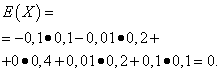
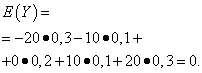
Example 12. Let the random variables x 1, x 2 be specified accordingly by the distribution laws:

x 1 Table 2

x 2 Table 3

Let's calculate M (x 1) and M (x 2)

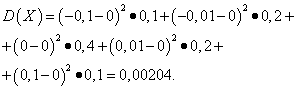
M (x 1) = (- 0.1) 0.1 + (- 0.01) 0.2 + 0 0.4 + 0.01 0.2 + 0.1 0.1 = 0

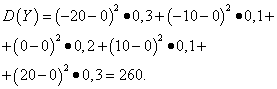
M (x 2) = (- 20) 0.3 + (- 10) 0.1 + 0 0.2 + 10 0.1 + 20 0.3 = 0

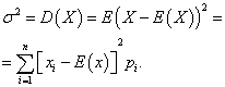
The mathematical expectations of both random variables are the same - they are equal to zero. However, the nature of their distribution is different. If the values ​​of x 1 differ little from their mathematical expectation, then the values ​​of x 2 differ to a large extent from their mathematical expectation, and the probabilities of such deviations are not small. These examples show that it is impossible to determine from the average value which deviations from it occur, both smaller and larger. So, with the same average annual precipitation in two areas, it cannot be said that these areas are equally favorable for agricultural work. Similarly, based on the average salary indicator, it is not possible to judge the share of high- and low-paid workers. Therefore, a numerical characteristic is introduced - dispersion D(x) , which characterizes the degree of deviation of a random variable from its average value:

D (x) = M (x - M (x)) 2 . (2)

Dispersion is the mathematical expectation of the squared deviation of a random variable from the mathematical expectation. For a discrete random variable, the variance is calculated using the formula:

D(x)= = (3)

From the definition of dispersion it follows that D (x) 0.

Dispersion properties:

1. The variance of the constant is zero

2. If a random variable is multiplied by a certain number k, then the variance will be multiplied by the square of this number

D (kx) = k 2 D (x)

3. D (x) = M (x 2) – M 2 (x)

4. For pairwise independent random variables x 1 , x 2 , … x n the variance of the sum is equal to the sum of the variances.

D (x 1 + x 2 + … + x n) = D (x 1) + D (x 2) +…+ D (x n)

Let's calculate the variance for the random variable from Example 11.

Mathematical expectation M (x) = 1. Therefore, according to formula (3) we have:

D (x) = (0 – 1) 2 1/4 + (1 – 1) 2 1/2 + (2 – 1) 2 1/4 =1 1/4 +1 1/4= 1/2

Note that it is easier to calculate variance if you use property 3:

D (x) = M (x 2) – M 2 (x).

Let's calculate the variances for the random variables x 1 , x 2 from Example 12 using this formula. The mathematical expectations of both random variables are zero.

D (x 1) = 0.01 0.1 + 0.0001 0.2 + 0.0001 0.2 + 0.01 0.1 = 0.001 + 0.00002 + 0.00002 + 0.001 = 0.00204

D (x 2) = (-20) 2 0.3 + (-10) 2 0.1 + 10 2 0.1 + 20 2 0.3 = 240 +20 = 260

The closer the variance value is to zero, the smaller the spread of the random variable relative to the mean value.

The quantity is called standard deviation. Random variable mode x discrete type Md The value of a random variable that has the highest probability is called.

Random variable mode x continuous type Md, is a real number defined as the point of maximum of the probability distribution density f(x).

Median of a random variable x continuous type Mn is a real number that satisfies the equation

There will also be problems for you to solve on your own, to which you can see the answers.

Expectation and variance are the most commonly used numerical characteristics of a random variable. They characterize the most important features of the distribution: its position and degree of scattering. The expected value is often called simply the average. random variable. Dispersion of a random variable - characteristic of dispersion, spread of a random variable about its mathematical expectation.

In many practical problems, a complete, exhaustive characteristic of a random variable - the distribution law - either cannot be obtained or is not needed at all. In these cases, one is limited to an approximate description of a random variable using numerical characteristics.

Expectation of a discrete random variable

Let's come to the concept of mathematical expectation. Let the mass of some substance be distributed between the points of the x-axis x1 , x 2 , ..., x n. Moreover, each material point has a corresponding mass with a probability of p1 , p 2 , ..., p n. It is required to select one point on the abscissa axis, characterizing the position of the entire system of material points, taking into account their masses. It is natural to take the center of mass of the system of material points as such a point. This is the weighted average of the random variable X, to which the abscissa of each point xi enters with a “weight” equal to the corresponding probability. The average value of the random variable obtained in this way X is called its mathematical expectation.

The mathematical expectation of a discrete random variable is the sum of the products of all its possible values ​​and the probabilities of these values:

Example 1. A win-win lottery has been organized. There are 1000 winnings, of which 400 are 10 rubles. 300 - 20 rubles each. 200 - 100 rubles each. and 100 - 200 rubles each. What is the average winnings for someone who buys one ticket?

Solution. We will find the average winnings if we divide the total amount of winnings, which is 10*400 + 20*300 + 100*200 + 200*100 = 50,000 rubles, by 1000 (total amount of winnings). Then we get 50000/1000 = 50 rubles. But the expression for calculating the average winnings can be presented in the following form:

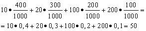
On the other hand, in these conditions, the winning amount is a random variable, which can take values ​​of 10, 20, 100 and 200 rubles. with probabilities equal to 0.4, respectively; 0.3; 0.2; 0.1. Therefore, the expected average win is equal to the sum of the products of the size of the wins and the probability of receiving them.

Example 2. The publisher decided to publish a new book. He plans to sell the book for 280 rubles, of which he himself will receive 200, 50 - the bookstore and 30 - the author. The table provides information about the costs of publishing a book and the probability of selling a certain number of copies of the book.

Find the publisher's expected profit.

Solution. The random variable “profit” is equal to the difference between the income from sales and the cost of costs. For example, if 500 copies of a book are sold, then the income from the sale is 200 * 500 = 100,000, and the cost of publication is 225,000 rubles. Thus, the publisher faces a loss of 125,000 rubles. The following table summarizes the expected values ​​of the random variable - profit:

Number	Profit xi	Probability pi	xi p i
500	-125000	0,20	-25000
1000	-50000	0,40	-20000
2000	100000	0,25	25000
3000	250000	0,10	25000
4000	400000	0,05	20000
Total:		1,00	25000

Thus, we obtain the mathematical expectation of the publisher’s profit:

.

Example 3. Probability of hitting with one shot p= 0.2. Determine the consumption of projectiles that provide a mathematical expectation of the number of hits equal to 5.

Solution. From the same mathematical expectation formula that we have used so far, we express x- shell consumption:

.

Example 4. Determine the mathematical expectation of a random variable x number of hits with three shots, if the probability of a hit with each shot p = 0,4 .

Hint: find the probability of random variable values ​​by Bernoulli's formula .

Properties of mathematical expectation

Let's consider the properties of mathematical expectation.

Property 1. The mathematical expectation of a constant value is equal to this constant:

Property 2. The constant factor can be taken out of the mathematical expectation sign:

Property 3. The mathematical expectation of the sum (difference) of random variables is equal to the sum (difference) of their mathematical expectations:

Property 4. The mathematical expectation of a product of random variables is equal to the product of their mathematical expectations:

Property 5. If all values ​​of a random variable X decrease (increase) by the same number WITH, then its mathematical expectation will decrease (increase) by the same number:

When you can’t limit yourself only to mathematical expectation

In most cases, only the mathematical expectation cannot sufficiently characterize a random variable.

Let the random variables X And Y are given by the following distribution laws:

Meaning X	Probability
-0,1	0,1
-0,01	0,2
0	0,4
0,01	0,2
0,1	0,1

Meaning Y	Probability
-20	0,3
-10	0,1
0	0,2
10	0,1
20	0,3

The mathematical expectations of these quantities are the same - equal to zero:

However, their distribution patterns are different. Random value X can only take values ​​that differ little from the mathematical expectation, and the random variable Y can take values ​​that deviate significantly from the mathematical expectation. A similar example: the average wage does not make it possible to judge the share of high- and low-paid workers. In other words, one cannot judge from the mathematical expectation what deviations from it, at least on average, are possible. To do this, you need to find the variance of the random variable.

Variance of a discrete random variable

Variance discrete random variable X is called the mathematical expectation of the square of its deviation from the mathematical expectation:

The standard deviation of a random variable X the arithmetic value of the square root of its variance is called:

.

Example 5. Calculate variances and standard deviations of random variables X And Y, the distribution laws of which are given in the tables above.

Solution. Mathematical expectations of random variables X And Y, as found above, are equal to zero. According to the dispersion formula at E(X)=E(y)=0 we get:

Then the standard deviations of random variables X And Y make up

.

Thus, with the same mathematical expectations, the variance of the random variable X very small, but a random variable Y- significant. This is a consequence of differences in their distribution.

Example 6. The investor has 4 alternative investment projects. The table summarizes the expected profit in these projects with the corresponding probability.

Project 1	Project 2	Project 3	Project 4
500, P=1	1000, P=0,5	500, P=0,5	500, P=0,5
	0, P=0,5	1000, P=0,25	10500, P=0,25
		0, P=0,25	9500, P=0,25

Find the mathematical expectation, variance and standard deviation for each alternative.

Solution. Let us show how these values ​​are calculated for the 3rd alternative:

The table summarizes the found values ​​for all alternatives.

All alternatives have the same mathematical expectations. This means that in the long run everyone has the same income. Standard deviation can be interpreted as a measure of risk - the higher it is, the greater the risk of the investment. An investor who does not want much risk will choose project 1 since it has the smallest standard deviation (0). If the investor prefers risk and high returns in a short period, then he will choose the project with the largest standard deviation - project 4.

Dispersion properties

Let us present the properties of dispersion.

Property 1. The variance of a constant value is zero:

Property 2. The constant factor can be taken out of the dispersion sign by squaring it:

.

Property 3. The variance of a random variable is equal to the mathematical expectation of the square of this value, from which the square of the mathematical expectation of the value itself is subtracted:

,

Where .

Property 4. The variance of the sum (difference) of random variables is equal to the sum (difference) of their variances:

Example 7. It is known that a discrete random variable X takes only two values: −3 and 7. In addition, the mathematical expectation is known: E(X) = 4 . Find the variance of a discrete random variable.

Solution. Let us denote by p the probability with which a random variable takes a value x1 = −3 . Then the probability of the value x2 = 7 will be 1 − p. Let us derive the equation for the mathematical expectation:

E(X) = x 1 p + x 2 (1 − p) = −3p + 7(1 − p) = 4 ,

where we get the probabilities: p= 0.3 and 1 − p = 0,7 .

Law of distribution of a random variable:

X	−3	7
p	0,3	0,7

We calculate the variance of this random variable using the formula from property 3 of dispersion:

D(X) = 2,7 + 34,3 − 16 = 21 .

Find the mathematical expectation of a random variable yourself, and then look at the solution

Example 8. Discrete random variable X takes only two values. It accepts the greater of the values ​​3 with probability 0.4. In addition, the variance of the random variable is known D(X) = 6 . Find the mathematical expectation of a random variable.

Example 9. There are 6 white and 4 black balls in the urn. 3 balls are drawn from the urn. The number of white balls among the drawn balls is a discrete random variable X. Find the mathematical expectation and variance of this random variable.

Solution. Random value X can take values ​​0, 1, 2, 3. The corresponding probabilities can be calculated from probability multiplication rule. Law of distribution of a random variable:

X	0	1	2	3
p	1/30	3/10	1/2	1/6

Hence the mathematical expectation of this random variable:

M(X) = 3/10 + 1 + 1/2 = 1,8 .

The variance of a given random variable is:

D(X) = 0,3 + 2 + 1,5 − 3,24 = 0,56 .

Expectation and variance of a continuous random variable

For a continuous random variable, the mechanical interpretation of the mathematical expectation will retain the same meaning: the center of mass for a unit mass distributed continuously on the x-axis with density f(x). Unlike a discrete random variable, whose function argument xi changes abruptly; for a continuous random variable, the argument changes continuously. But the mathematical expectation of a continuous random variable is also related to its average value.

To find the mathematical expectation and variance of a continuous random variable, you need to find definite integrals . If the density function of a continuous random variable is given, then it directly enters into the integrand. If a probability distribution function is given, then by differentiating it, you need to find the density function.

The arithmetic average of all possible values ​​of a continuous random variable is called its mathematical expectation, denoted by or .

Expected value

Dispersion continuous random variable X, the possible values ​​of which belong to the entire Ox axis, is determined by the equality:

Purpose of the service. The online calculator is designed to solve problems in which either distribution density f(x) or distribution function F(x) (see example). Usually in such tasks you need to find mathematical expectation, standard deviation, plot functions f(x) and F(x).

Instructions. Select the type of source data: distribution density f(x) or distribution function F(x).

The distribution density f(x) is given:

The distribution function F(x) is given:

A continuous random variable is specified by a probability density
(Rayleigh distribution law - used in radio engineering). Find M(x) , D(x) .

The random variable X is called continuous , if its distribution function F(X)=P(X< x) непрерывна и имеет производную.
The distribution function of a continuous random variable is used to calculate the probability of a random variable falling into a given interval:
P(α< X < β)=F(β) - F(α)
Moreover, for a continuous random variable, it does not matter whether its boundaries are included in this interval or not:
P(α< X < β) = P(α ≤ X < β) = P(α ≤ X ≤ β)
Distribution density a continuous random variable is called a function
f(x)=F’(x) , derivative of the distribution function.

Properties of distribution density

1. The distribution density of the random variable is non-negative (f(x) ≥ 0) for all values ​​of x.
2. Normalization condition:

The geometric meaning of the normalization condition: the area under the distribution density curve is equal to unity.
3. The probability of a random variable X falling into the interval from α to β can be calculated using the formula

Geometrically, the probability of a continuous random variable X falling into the interval (α, β) is equal to the area of ​​the curvilinear trapezoid under the distribution density curve based on this interval.
4. The distribution function is expressed in terms of density as follows:

The value of the distribution density at point x is not equal to the probability of accepting this value; for a continuous random variable we can only talk about the probability of falling into a given interval. Let )