home / Relationship/ Scientific forum dxdy. Basic properties of the roots of an algebraic equation Examples of determining the roots of a quadratic equation

Scientific forum dxdy. Basic properties of the roots of an algebraic equation Examples of determining the roots of a quadratic equation

Formulas for the roots of a quadratic equation. The cases of real, multiple and complex roots are considered. Factoring a quadratic trinomial. Geometric interpretation. Examples of determining roots and factoring.

Content

See also: Solving quadratic equations online

Basic formulas

Consider the quadratic equation:
(1) .
Roots of a quadratic equation(1) are determined by the formulas:
; .
These formulas can be combined like this:
.
When the roots of a quadratic equation are known, then a polynomial of the second degree can be represented as a product of factors (factored):
.

Next we assume that are real numbers.
Let's consider discriminant of a quadratic equation:
.
If the discriminant is positive, then the quadratic equation (1) has two different real roots:
; .
Then the factorization of the quadratic trinomial has the form:
.
If the discriminant is equal to zero, then the quadratic equation (1) has two multiple (equal) real roots:
.
Factorization:
.
If the discriminant is negative, then the quadratic equation (1) has two complex conjugate roots:
;
.
Here is the imaginary unit, ;
and are the real and imaginary parts of the roots:
; .
Then

.

Graphic interpretation

If you plot the function
,
which is a parabola, then the points of intersection of the graph with the axis will be the roots of the equation
.
When , the graph intersects the x-axis (axis) at two points ().
When , the graph touches the x-axis at one point ().
When , the graph does not intersect the x-axis ().

Useful formulas related to quadratic equation

(f.1) ;
(f.2) ;
(f.3) .

Derivation of the formula for the roots of a quadratic equation

We carry out transformations and apply formulas (f.1) and (f.3):

,
Where
; .

So, we got the formula for a polynomial of the second degree in the form:
.
This shows that the equation

performed at
And .
That is, and are the roots of the quadratic equation
.

Examples of determining the roots of a quadratic equation

Example 1

(1.1) .

.
Comparing with our equation (1.1), we find the values of the coefficients:
.
We find the discriminant:
.
Since the discriminant is positive, the equation has two real roots:
;
;
.

From here we obtain the factorization of the quadratic trinomial:

.

Graph of the function y = 2 x 2 + 7 x + 3 intersects the x-axis at two points.

Let's plot the function
.
The graph of this function is a parabola. It crosses the abscissa axis (axis) at two points:
And .
These points are the roots of the original equation (1.1).

;
;
.

Example 2

Find the roots of a quadratic equation:
(2.1) .

Let's write the quadratic equation in general form:
.
Comparing with the original equation (2.1), we find the values of the coefficients:
.
We find the discriminant:
.
Since the discriminant is zero, the equation has two multiple (equal) roots:
;
.

Then the factorization of the trinomial has the form:
.

Graph of the function y = x 2 - 4 x + 4 touches the x-axis at one point.

Let's plot the function
.
The graph of this function is a parabola. It touches the x-axis (axis) at one point:
.
This point is the root of the original equation (2.1). Because this root is factored twice:
,
then such a root is usually called a multiple. That is, they believe that there are two equal roots:
.

;
.

Example 3

Find the roots of a quadratic equation:
(3.1) .

Let's write the quadratic equation in general form:
(1) .
Let's rewrite the original equation (3.1):
.
Comparing with (1), we find the values of the coefficients:
.
We find the discriminant:
.
The discriminant is negative, . Therefore there are no real roots.

You can find complex roots:
;
;
.

Then

.

The graph of the function does not cross the x-axis. There are no real roots.

Let's plot the function
.
The graph of this function is a parabola. It does not intersect the x-axis (axis). Therefore there are no real roots.

There are no real roots. Complex roots:
;
;
.

INTRODUCTION

The computing technology of today provides powerful tools for actually doing the work of counting. Thanks to this, in many cases it became possible to abandon the approximate interpretation of applied issues and move on to solving problems in an exact formulation. Reasonable use of modern computer technology is inconceivable without the skillful application of methods of approximate and numerical analysis.

Numerical methods are aimed at solving problems that arise in practice. Solving a problem using numerical methods comes down to arithmetic and logical operations on numbers, which requires the use of computer technology, such as spreadsheet processors of modern office programs for personal computers.

The goal of the “Numerical Methods” discipline is to find the most effective method for solving a specific problem.

Solving algebraic equations is one of the essential problems of applied analysis, the need for which arises in numerous and diverse sections of physics, mechanics, technology and natural science in the broad sense of the word.

This course project is devoted to one of the methods for solving algebraic equations - the Lobachevsky-Greffe method.

The purpose of this work is to consider the idea of the Lobachevsky–Greffe method for solving algebraic problems, and to provide a computational scheme for finding real roots using MS Office Excel. The project examines the main theoretical issues related to finding the roots of algebraic equations using the Lobachevsky–Greffe method. The practical part of this work presents solutions to algebraic equations using the Lobachevsky–Greffe method.

1 THEORETICAL PART

1.1 Problem statement

Let a set X of elements x and a set Y with elements y be given. Let us also assume that an operator is defined on the set X, which assigns to each element x from X some element y from Y. Take some element

and set ourselves the goal of finding such elements

, for which

is an image.

This problem is equivalent to solving the equation

(1.1)

The following problems can be posed for it.

Conditions for the existence of a solution to the equation.
Condition for the uniqueness of a solution to the equation.
A solution algorithm, following which, it would be possible to find, depending on the goal and conditions, exactly or approximately all solutions to equation (1.1), or any one solution specified in advance, or any of the existing ones.

Next, we will consider equations in which x and y will be numerical quantities, X, Y will be sets of their values, and the operator

there will be some function. In this case, equation (1.1) can be written in the form

(1.2)

In the theory of numerical methods, one strives to construct a computational process with the help of which one can find a solution to equation (1.2) with a predetermined accuracy. Convergent processes are especially important, making it possible to solve the equation with any error, no matter how small.

Our task is to find, generally speaking, approximately, the element . For this purpose, an algorithm is being developed that produces a sequence of approximate solutions

, and in such a way that the relation holds

1.2 Algebraic equations

1.2.1 Basic concepts about algebraic equation

Consider an algebraic equation of nth degree

where are the coefficients
are real numbers, and
.

Theorem 1.1 (fundamental theorem of algebra). The algebraic equation of the nth degree (1.3) has exactly n roots, real and complex, provided that each root is counted as many times as its multiplicity.

In this case, they say that the root of equation (1.3) has multiplicity s if
,
.

The complex roots of equation (1.3) have the property of pairwise conjugacy.

Theorem 1.2. If the coefficients of the algebraic equation (1.3) are real, then the complex roots of this equation are pairwise complex conjugate, i.e. If
(
are real numbers) is the root of equation (1.3), of multiplicity s, then the number
is also the root of this equation and has the same multiplicity s.

Consequence. An algebraic equation of odd degree with real coefficients has at least one real root.

1.2.2 Roots of an algebraic equation

are the roots of equation (1.3), then the left-hand side has the following expansion:
. (1.6)
By multiplying the binomials in formula (1.6) and equating the coefficients at the same powers of x on the left and right sides of equality (1.6), we obtain the relationships between the roots and coefficients of the algebraic equation (1.3):

(1.7)
If we take into account the multiplicities of the roots, then expansion (1.6) takes the form
,
Where

–different roots of equation (1) and

– their multiplicity, and

Derivative
is expressed as follows:

where Q(x) is a polynomial such that

at k=1,2,…,m

Therefore the polynomial

is the greatest common divisor of the polynomial

and its derivative

, and can be found using the Euclidean algorithm. Let's make a quotient

,
and we get a polynomial

with real odds

, A 1 , A 2 ,…, A m , whose roots

are different.

Thus, solving an algebraic equation with multiple roots reduces to solving a lower order algebraic equation with different roots.

1.2.3 Number of real roots of a polynomial

A general idea of the number of real roots of equation (1.3) on the interval (a,b) is given by the graph of the function

, where the roots

are the abscissas of the points of intersection of the graph with the Ox axis.

Let us note some properties of the polynomial P(x):

If P(a)P(b)
If P(a)P(b)>0, then on the interval (a, b) there is an even number or no roots of the polynomial P(x).

The question of the number of real roots of an algebraic equation on a given interval is solved by the Sturm method.

Definition. Let an ordered finite system of non-zero real numbers be given:

,…,

(1.9)
They say that for a pair of adjacent elements

system (1.9) there is a sign change if these elements have opposite signs, i.e.

,
and there is no change in sign if their signs are the same, i.e.

.
Definition. Total number of sign changes of all pairs of adjacent elements

system (1.9) is called the number of sign changes in system (1.9).

Definition. For a given polynomial P(x), the Sturm system is the system of polynomials

,…,

Where
, – the remainder taken with the opposite sign when dividing a polynomial by , – the remainder taken with the opposite sign when dividing a polynomial by, etc.

Remark 1. If a polynomial has no multiple roots, then the last element of the Sturm system is a nonzero real number.

Remark 2. The elements of the Sturm system can be calculated up to a positive numerical factor.

Let us denote by N(c) the number of sign changes in the Sturm system at x=c, provided that the zero elements of this system are crossed out.

Theorem 1.5. (Sturm's theorem). If the polynomial P(x) has no multiple horses and
,
, then the number of its real roots
on the interval
exactly equal to the number of lost sign changes in the Sturm system of the polynomial
when moving from
before
, i.e.

.
Corollary 1. If

, then the number

positive and number

negative roots of the polynomial are respectively equal

.
Corollary 2. In order for all the roots of a polynomial P(x) of degree n, which has no multiple roots, to be real, it is necessary and sufficient that the condition be satisfied
.
Thus, in equation (1.3) all roots will be valid if and only if:

Using the Sturm system, you can separate the roots of an algebraic equation by dividing the interval (a,b), containing all the real roots of the equation, into a finite number of partial intervals

such that

1.3 Lobachevsky–Greffe method for approximate solution of algebraic equations

1.3.1 Idea of the method

Consider the algebraic equation (1.3).

Let's pretend that

, (1.15)
those. the roots are different in modulus, and the modulus of each previous root is significantly greater than the modulus of the next one. In other words, let us assume that the ratio of any two adjacent roots, counting in descending order of their numbers, is a quantity that is small in absolute value:

, (1.16)

Where
And – small value. Such roots are called separated.

(1.17)
Where , ,…, – quantities that are small in absolute value compared to unity. Neglecting in system (1.17) the quantities
, we will have approximate relations

(1.18)
Where do we find roots?

(1.19)
The accuracy of the roots in the system of equalities (1.20) depends on how small in absolute value the quantities in relations (1.16)

To achieve separation of the roots, based on equation (1.3), they compose the transformed equation

, (1.20)
whose roots

,…,

are the m-e powers of the roots

,…,

equation (1.3).

If all the roots of equation (1.3) are different and their modules satisfy condition (1.17), then for a sufficiently large m the roots , ,..., of equation (1.20) will be separated, because

.
Obviously, it is enough to construct an algorithm for finding an equation whose roots will be the squares of the roots of the given equation. Then it will be possible to obtain an equation whose roots will be equal to the roots of the original equation to the power

1.3.2 Squaring roots

We write the polynomial (1.3) in the following form

And multiply it by a polynomial of the form

Then we get

Having made a replacement

and multiplying by

, will have
. (1.21)
The roots of the polynomial (1.21) are related to the roots of the polynomial (1.3) by the following relation

.
Therefore, the equation we are interested in is
,
whose coefficients are calculated using formula (1.22)

, (1.22)
where it is assumed that

Applying successively k times the process of squaring the roots to the polynomial (1.3), we obtain the polynomial

, (1.23)
in which

, etc.

For sufficiently large k, it is possible to ensure that the roots of equation (1.23) satisfy the system

(1.24)
Let us determine the number k for which system (1.24) is satisfied with a given accuracy.

Let us assume that the required k has already been achieved and equalities (1.24) are satisfied with the accepted accuracy. Let's do one more transformation and find the polynomial

,
for which system (1.24) also holds for

Since by virtue of formula (1.22)

, (1.25)
then, substituting (1.25) into system (1.24), we obtain that the absolute values of the coefficients

must be equal to the accepted accuracy of the squares of the coefficients

. The fulfillment of these equalities will indicate that the required value of k has already been achieved at the kth step.

Thus, squaring the roots of equation (1.3) should be stopped if, in the accepted accuracy, only the squared coefficients are retained on the right side of formula (1.24), and the doubled sum of the products is below the accuracy limit.

Then the real roots of the equation are separated and their modules are found by the formula

(1.26)
The sign of the root can be determined by a rough estimate by substituting the values And
into equation (1.3).

2 PRACTICAL PART

2.1 Task 1

. (2.1)
First, let's establish the number of real and complex roots in equation (2.1). To do this, we will use Sturm’s theorem.

The Sturm system for equation (2.1) will have the following form:

Where do we get it from?
Table 2.1.

Polynomial	Points on the real axis
Polynomial
	+	+
	–	+
	–	–
	–	+
	–	–
Number of sign changes	1	3

Thus, we find that the number of real roots in equation (2.1) is equal to
,
those. equation (2.1) contains 2 real and two complex roots.

To find the roots of the equation, we use the Lobachevsky–Greffe method for a pair of complex conjugate roots.

Let's square the roots of the equation. The coefficients were calculated using the following formula

, (2.2)
Where

, (2.3)
A
considered equal to 0 when
.

The results of calculations with eight significant figures are given in Table 2.2

Table 2.2.

i	0	1	2	3	4

	0	-3.8000000E+01	3.5400000E+02	3.8760000E+03	0
	1	4.3000000E+01	7.1500000E+02	4.8370000E+03	1.0404000E+04

	0	-1.4300000E+03	-3.9517400E+05	-1.4877720E+07	0
	1	4.1900000E+02	1.1605100E+05	8.5188490E+06	1.0824322E+08

	0	-2.3210200E+05	-6.9223090E+09	-2.5123467E+13	0
	1	-5.6541000E+04	6.5455256E+09	4.7447321E+13	1.1716594E+16

	0	-1.3091051E+10	5.3888712E+18	-1.5338253E+26	0
	1	-9.8941665E+09	4.8232776E+19	2.0978658E+27	1.3727857E+32

	0	-9.6465552E+19	4.1513541E+37	-1.3242653E+52	0
	1	1.4289776E+18	2.3679142E+39	4.3877982E+54	1.8845406E+64

	0	-4.7358285E+39	-1.2540130E+73	-8.9248610+103	0
	1	-4.7337865E+39	5.6070053E+78	1.9252683+109	3.5514932+128

	0	-1.1214011E+79	1.8227619+149	-3.9826483+207	0
	1	1.1194724E+79	3.1438509+157	3.7066582+218	1.2613104+257

As can be seen from Table 2.2 at the 7th step the roots , (counting in descending order of modules) can be considered separated. We find the moduli of the roots using formula (1.27) and determine their sign using a rough estimate:

Since the converted coefficient at changes sign, then this equation has complex roots, which are determined from equation (1.31) using formulas (1.29) and (1.30):

2.2 Task 2

Using the Lobachevsky–Greffe method, solve the equation:
. (2.4)
To begin with, using Sturm’s theorem, we determine the number of real and complex roots in equation (2.2).

For this equation, the Sturm system has the form

Where do we get it from?

Table 2.3.

Polynomial	Points on the real axis
Polynomial
	+	+
	–	+
	+	+
	–	+
	–	–
Number of sign changes	3	1

Thus, we find that the number of real roots in equation (2.2) is equal to

,
those. equation (2.2) contains 2 real and two complex roots.

To approximately find the roots of the equation, we will use the Lobachevsky–Greffe method for a pair of complex conjugate roots.

Let's square the roots of the equation. We will calculate the coefficients using formulas (2.2) and (2.3).

The results of calculations with eight significant figures are given in Table 2.4

Table 2.4.
-1.8886934E+24 4.6649263E+47 i.
The relative error of the roots, calculated using formula (1.28) is equal to
,

2.4 Analysis of the results obtained

From the equations obtained when solving equations (2.1) and (2.4), one can judge the following features of the Lobachevsky–Greffe method.

Using the method under consideration, you can find all the roots of a polynomial with fairly high accuracy, with a small number of iterations.

The magnitude of the error of the resulting roots depends to a high degree on the separation of the roots in the original polynomial, for example, in equation (2.1) the minimum difference between roots of different modulus is equal to
And
in equation (2.4), which results in errors of different orders (4.52958089E–11 and 4.22229789E–06, respectively) for the same number of iterations.

Thus, the Lobachevsky–Greffe method gives good accuracy for separated roots, and significantly loses for multiple or similar roots.

CONCLUSION

The Lobachevsky–Greffe method, which was considered in this project, has a simple calculation scheme and allows using Excel to find with great accuracy the modulus of all roots of an algebraic equation,

The Lobachevsky–Graeffe method is one of the most effective calculation methods, which, with a small number of iterations, gives results with fairly good accuracy, so the scope of use of this method in practice is very wide. The method can be used in constructing mathematical models of chemical and physical processes and in optimization methods.

LIST OF LINKS

1. V.P. Demidovich, I.A. Maroon. Fundamentals of computational mathematics. – M.: Nauka, 1966.–664 p.

2. V.L. Zaguskin. Handbook on numerical methods for solving algebraic and transcendental equations. – M.: State Publishing House of Physical and Mathematical Literature, 1960.–216 pp.

3. V.I. Krylov, V.V. Bobkov, P.I. Monastic. Computational methods of higher mathematics. – Minsk: Higher School, 1972, vol. 1.–584 p.

4. A.G. Kurosh. Course of higher algebra. – M.: Nauka, 1971, – 432 p.

5. Yu.I. Ryzhikov. Fortran programming PowerStation for engineers. Practical guide. – St. Petersburg: CORONA print, 1999. – 160 p.

i	0	1	2	3	4

	0	-9.2000000E+00	-3.3300000E+01	1.3800000E+02	0

Examples (number of roots of an algebraic equation)

1) x 2 – 4x+ 5 = 0 - algebraic equation of the second degree (quadratic equation) 
2
= 2 i- two roots;

2) x 3 + 1 = 0 - algebraic equation of the third degree (binomial equation) 

;

3) P 3 (x) = x 3 + x 2 – x– 1 = 0 – algebraic equation of the third degree;

number x 1 = 1 is its root, since P 3 (1) 0, therefore, by Bezout’s theorem
; divide the polynomial P 3 (x) by binomial ( x– 1) “in a column”:


								x 2 + 2x +1

original equation P 3 (x) = x 3 + x 2 – x – 1 = 0 

(x – 1)(x 2 + 2x + 1) = 0  (x – 1)(x + 1) 2 = 0  x 1 = 1 - simple root, x 2 = –1 - double root.

Property 2 (about complex roots of an algebraic equation with real coefficients)

If an algebraic equation with real coefficients has complex roots, then these roots are always pair complex conjugate, that is, if the number
is the root of the equation
, then the number
is also the root of this equation.

 To prove it, you need to use the definition and the following easily verifiable properties of the complex conjugation operation:

If
, That
and the equalities are valid:

,
,
,
,

If
is a real number, then
.

Because
is the root of the equation
, That

Where
-- real numbers at
.

Let's take the conjugation from both sides of the last equality and use the listed properties of the conjugation operation:

, that is, the number
also satisfies the equation
, therefore, is its root

Examples (complex roots of algebraic equations with real coefficients)

As a consequence of the proven property about the pairing of complex roots of an algebraic equation with real coefficients, another property of polynomials is obtained.

 We will proceed from expansion (6) of the polynomial
to linear factors:

Let the number x 0 = a + bi- complex root of a polynomial P n (x), that is, this is one of the numbers
. If all the coefficients of this polynomial are real numbers, then the number
is also its root, that is, among the numbers
there is also a number
.

Let's calculate the product of binomials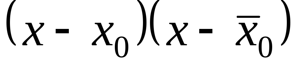
:

The result is a quadratic trinomial with real odds

Thus, any pair of binomials with complex conjugate roots in formula (6) leads to a quadratic trinomial with real coefficients. 

Examples (factorization of a polynomial with real coefficients)

1)P 3 (x) = x 3 + 1 = (x + 1)(x 2 – x + 1);

2)P 4 (x) = x 4 – x 3 + 4x 2 – 4x = x(x –1)(x 2 + 4).

Property 3 (on integer and rational roots of an algebraic equation with real integer coefficients)

Let us be given an algebraic equation

, all coefficients
which are real integers,

1. Let it be an integer is the root of the equation

Since the whole number
represented by the product of an integer and expressions that have an integer value.

2. Let the algebraic equation
has a rational root

, moreover, numbers p And q are relatively prime

.

This identity can be written in two versions:

From the first version of the notation it follows that
, and from the second – what
, since the numbers p And q are relatively prime.

Examples (selection of integer or rational roots of an algebraic equation with integer coefficients)

Etc. is of a general educational nature and is of great importance for studying the ENTIRE course of higher mathematics. Today we will repeat “school” equations, but not just “school” ones - but those that are found everywhere in various vyshmat problems. As usual, the story will be told in an applied way, i.e. I will not focus on definitions and classifications, but will share with you my personal experience of solving it. The information is intended primarily for beginners, but more advanced readers will also find many interesting points for themselves. And, of course, there will be new material that goes beyond high school.

So the equation…. Many remember this word with a shudder. What are the “sophisticated” equations with roots worth... ...forget about them! Because then you will meet the most harmless “representatives” of this species. Or boring trigonometric equations with dozens of solution methods. To be honest, I didn’t really like them myself... Don't panic! – then mostly “dandelions” await you with an obvious solution in 1-2 steps. Although the “burdock” certainly clings, you need to be objective here.

Oddly enough, in higher mathematics it is much more common to deal with very primitive equations like linear equations

What does it mean to solve this equation? This means finding SUCH value of “x” (root) that turns it into a true equality. Let’s throw the “three” to the right with a change of sign:

and drop the “two” to the right side (or, the same thing - multiply both sides by) :

To check, let’s substitute the won trophy into the original equation:

The correct equality is obtained, which means that the value found is indeed the root of this equation. Or, as they also say, satisfies this equation.

Please note that the root can also be written as a decimal fraction:
And try not to stick to this bad style! I repeated the reason more than once, in particular, at the very first lesson on higher algebra.

By the way, the equation can also be solved “in Arabic”:

And what’s most interesting is that this recording is completely legal! But if you are not a teacher, then it’s better not to do this, because originality is punishable here =)

And now a little about

graphical solution method

The equation has the form and its root is "X" coordinate intersection points linear function graph with the graph of a linear function (x axis):

It would seem that the example is so elementary that there is nothing more to analyze here, but one more unexpected nuance can be “squeezed” out of it: let’s present the same equation in the form and construct graphs of the functions:

Wherein, please don't confuse the two concepts: an equation is an equation, and function– this is a function! Functions only help find the roots of the equation. Of which there may be two, three, four, or even infinitely many. The closest example in this sense is the well-known quadratic equation, the solution algorithm for which received a separate paragraph "hot" school formulas. And this is no coincidence! If you can solve a quadratic equation and know Pythagorean theorem, then, one might say, “half of higher mathematics is already in your pocket” =) Exaggerated, of course, but not so far from the truth!

Therefore, let’s not be lazy and solve some quadratic equation using standard algorithm:

, which means the equation has two different valid root:

It is easy to verify that both found values actually satisfy this equation:

What to do if you suddenly forgot the solution algorithm, and there are no means/helping hands at hand? This situation may arise, for example, during a test or exam. We use the graphical method! And there are two ways: you can build point by point parabola , thereby finding out where it intersects the axis (if it crosses at all). But it’s better to do something more cunning: imagine the equation in the form, draw graphs of simpler functions - and "X" coordinates their points of intersection are clearly visible!

If it turns out that the straight line touches the parabola, then the equation has two matching (multiple) roots. If it turns out that the straight line does not intersect the parabola, then there are no real roots.

To do this, of course, you need to be able to build graphs of elementary functions, but on the other hand, even a schoolchild can do these skills.

And again - an equation is an equation, and functions , are functions that only helped solve the equation!

And here, by the way, it would be appropriate to remember one more thing: if all the coefficients of an equation are multiplied by a non-zero number, then its roots will not change.

So, for example, the equation has the same roots. As a simple “proof”, I’ll take the constant out of brackets:
and I’ll remove it painlessly (I will divide both parts by “minus two”):

BUT! If we consider the function , then you can’t get rid of the constant here! It is only permissible to take the multiplier out of brackets: .

Many people underestimate the graphical solution method, considering it something “undignified,” and some even completely forget about this possibility. And this is fundamentally wrong, since plotting graphs sometimes just saves the situation!

Another example: suppose you don’t remember the roots of the simplest trigonometric equation: . The general formula is in school textbooks, in all reference books on elementary mathematics, but they are not available to you. However, solving the equation is critical (aka “two”). There is an exit! – build graphs of functions:

after which we calmly write down the “X” coordinates of their intersection points:

There are infinitely many roots, and in algebra their condensed notation is accepted:
, Where ( – set of integers) .

And, without “going away”, a few words about the graphical method for solving inequalities with one variable. The principle is the same. So, for example, the solution to the inequality is any “x”, because The sinusoid lies almost completely under the straight line. The solution to the inequality is the set of intervals in which the pieces of the sinusoid lie strictly above the straight line (x-axis):

or, in short:

But here are the many solutions to the inequality: empty, since no point of the sinusoid lies above the straight line.

Is there anything you don't understand? Urgently study the lessons about sets And function graphs!

Let's warm up:

Exercise 1

Solve the following trigonometric equations graphically:

Answers at the end of the lesson

As you can see, to study exact sciences it is not at all necessary to cram formulas and reference books! Moreover, this is a fundamentally flawed approach.

As I already reassured you at the very beginning of the lesson, complex trigonometric equations in a standard course of higher mathematics have to be solved extremely rarely. All complexity, as a rule, ends with equations like , the solution of which is two groups of roots originating from the simplest equations and . Don’t worry too much about solving the latter – look in a book or find it on the Internet =)

The graphical solution method can also help out in less trivial cases. Consider, for example, the following “ragtag” equation:

The prospects for its solution look... don’t look like anything at all, but you just have to imagine the equation in the form , build function graphs and everything will turn out to be incredibly simple. There is a drawing in the middle of the article about infinitesimal functions (will open in the next tab).

Using the same graphical method, you can find out that the equation already has two roots, and one of them is equal to zero, and the other, apparently, irrational and belongs to the segment . This root can be calculated approximately, for example, tangent method. By the way, in some problems, it happens that you don’t need to find the roots, but find out do they exist at all?. And here, too, a drawing can help - if the graphs do not intersect, then there are no roots.

Rational roots of polynomials with integer coefficients.
Horner scheme

And now I invite you to turn your gaze to the Middle Ages and feel the unique atmosphere of classical algebra. For a better understanding of the material, I recommend that you read at least a little complex numbers.

They are the best. Polynomials.

The object of our interest will be the most common polynomials of the form with whole coefficients A natural number is called degree of polynomial, number – coefficient of the highest degree (or just the highest coefficient), and the coefficient is free member.

I will briefly denote this polynomial by .

Roots of a polynomial call the roots of the equation

I love iron logic =)

For examples, go to the very beginning of the article:

There are no problems with finding the roots of polynomials of the 1st and 2nd degrees, but as you increase this task becomes more and more difficult. Although on the other hand, everything is more interesting! And this is exactly what the second part of the lesson will be devoted to.

First, literally half the screen of theory:

1) According to the corollary fundamental theorem of algebra, the degree polynomial has exactly complex roots. Some roots (or even all) may be particularly valid. Moreover, among the real roots there may be identical (multiple) roots (minimum two, maximum pieces).

If some complex number is the root of a polynomial, then conjugate its number is also necessarily the root of this polynomial (conjugate complex roots have the form ).

The simplest example is a quadratic equation, which was first encountered in 8 (like) class, and which we finally “finished off” in the topic complex numbers. Let me remind you: a quadratic equation has either two different real roots, or multiple roots, or conjugate complex roots.

2) From Bezout's theorem it follows that if a number is the root of an equation, then the corresponding polynomial can be factorized:
, where is a polynomial of degree .

And again, our old example: since is the root of the equation, then . After which it is not difficult to obtain the well-known “school” expansion.

The corollary of Bezout's theorem has great practical value: if we know the root of an equation of the 3rd degree, then we can represent it in the form and from the quadratic equation it is easy to find out the remaining roots. If we know the root of an equation of the 4th degree, then it is possible to expand the left side into a product, etc.

And there are two questions here:

Question one. How to find this very root? First of all, let's define its nature: in many problems of higher mathematics it is necessary to find rational, in particular whole roots of polynomials, and in this regard, further we will be mainly interested in them.... ...they are so good, so fluffy, that you just want to find them! =)

The first thing that comes to mind is the selection method. Consider, for example, the equation . The catch here is in the free term - if it were equal to zero, then everything would be fine - we take the “x” out of brackets and the roots themselves “fall out” to the surface:

But our free term is equal to “three”, and therefore we begin to substitute various numbers into the equation that claim to be “root”. First of all, the substitution of single values suggests itself. Let's substitute:

Received incorrect equality, thus, the unit “did not fit.” Well, okay, let's substitute:

Received true equality! That is, the value is the root of this equation.

To find the roots of a polynomial of the 3rd degree, there is an analytical method (the so-called Cardano formulas), but now we are interested in a slightly different task.

Since - is the root of our polynomial, the polynomial can be represented in the form and arises Second question: how to find a “younger brother”?

The simplest algebraic considerations suggest that to do this we need to divide by . How to divide a polynomial by a polynomial? The same school method that divides ordinary numbers - “column”! I discussed this method in detail in the first examples of the lesson. Complex Limits, and now we will look at another method, which is called Horner scheme.

First we write the “highest” polynomial with everyone , including zero coefficients:
, after which we enter these coefficients (strictly in order) into the top row of the table:

We write the root on the left:

I’ll immediately make a reservation that Horner’s scheme also works if the “red” number Not is the root of the polynomial. However, let's not rush things.

We remove the leading coefficient from above:

The process of filling the lower cells is somewhat reminiscent of embroidery, where “minus one” is a kind of “needle” that permeates the subsequent steps. We multiply the “carried down” number by (–1) and add the number from the top cell to the product:

We multiply the found value by the “red needle” and add the following equation coefficient to the product:

And finally, the resulting value is again “processed” with the “needle” and the upper coefficient:

The zero in the last cell tells us that the polynomial is divided into without a trace (as it should be), while the expansion coefficients are “removed” directly from the bottom line of the table:

Thus, we moved from the equation to an equivalent equation and everything is clear with the two remaining roots (in this case we get conjugate complex roots).

The equation, by the way, can also be solved graphically: plot "lightning" and see that the graph crosses the x-axis () at point . Or the same “cunning” trick - we rewrite the equation in the form , draw elementary graphs and detect the “X” coordinate of their intersection point.

By the way, the graph of any function-polynomial of the 3rd degree intersects the axis at least once, which means the corresponding equation has at least one valid root. This fact is true for any polynomial function of odd degree.

And here I would also like to dwell on important point which concerns terminology: polynomial And polynomial function – it's not the same thing! But in practice they often talk, for example, about the “graph of a polynomial,” which, of course, is negligence.

However, let's return to Horner's scheme. As I mentioned recently, this scheme works for other numbers, but if the number Not is the root of the equation, then a non-zero addition (remainder) appears in our formula:

Let’s “run” the “unsuccessful” value according to Horner’s scheme. In this case, it is convenient to use the same table - write a new “needle” on the left, move the leading coefficient from above (left green arrow), and off we go:

To check, let’s open the brackets and present similar terms:
, OK.

It is easy to see that the remainder (“six”) is exactly the value of the polynomial at . And in fact - what is it like:
, and even nicer - like this:

From the above calculations it is easy to understand that Horner’s scheme allows not only to factor the polynomial, but also to carry out a “civilized” selection of the root. I suggest you consolidate the calculation algorithm yourself with a small task:

Task 2

Using Horner's scheme, find the integer root of the equation and factor the corresponding polynomial

In other words, here you need to sequentially check the numbers 1, –1, 2, –2, ... – until a zero remainder is “drawn” in the last column. This will mean that the “needle” of this line is the root of the polynomial

It is convenient to arrange the calculations in a single table. Detailed solution and answer at the end of the lesson.

The method of selecting roots is good for relatively simple cases, but if the coefficients and/or degree of the polynomial are large, then the process may take a long time. Or maybe there are some values from the same list 1, –1, 2, –2 and there is no point in considering? And, besides, the roots may turn out to be fractional, which will lead to a completely unscientific poking.

Fortunately, there are two powerful theorems that can significantly reduce the search for “candidate” values for rational roots:

Theorem 1 Let's consider irreducible fraction , where . If the number is the root of the equation, then the free term is divided by and the leading coefficient is divided by.

In particular, if the leading coefficient is , then this rational root is an integer:

And we begin to exploit the theorem with just this tasty detail:

Let's return to the equation. Since its leading coefficient is , then hypothetical rational roots can be exclusively integer, and the free term must necessarily be divided into these roots without a remainder. And “three” can only be divided into 1, –1, 3 and –3. That is, we have only 4 “root candidates”. And, according to Theorem 1, other rational numbers cannot be roots of this equation IN PRINCIPLE.

There are a little more “contenders” in the equation: the free term is divided into 1, –1, 2, – 2, 4 and –4.

Please note that the numbers 1, –1 are “regulars” of the list of possible roots (an obvious consequence of the theorem) and the best choice for priority testing.

Let's move on to more meaningful examples:

Problem 3

Solution: since the leading coefficient is , then hypothetical rational roots can only be integer, and they must necessarily be divisors of the free term. “Minus forty” is divided into the following pairs of numbers:
– a total of 16 “candidates”.

And here a tempting thought immediately appears: is it possible to weed out all the negative or all the positive roots? In some cases it is possible! I will formulate two signs:

1) If All If the coefficients of the polynomial are non-negative or all non-positive, then it cannot have positive roots. Unfortunately, this is not our case (Now, if we were given an equation - then yes, when substituting any value of the polynomial, the value of the polynomial is strictly positive, which means that all positive numbers (and irrational ones too) cannot be roots of the equation.

2) If the coefficients for odd powers are non-negative, and for all even powers (including free member) are negative, then the polynomial cannot have negative roots. Or “mirror”: the coefficients for odd powers are non-positive, and for all even powers they are positive.

This is our case! Looking a little closer, you can see that when substituting any negative “X” into the equation, the left-hand side will be strictly negative, which means that negative roots disappear

Thus, there are 8 numbers left for research:

We “charge” them sequentially according to Horner’s scheme. I hope you have already mastered mental calculations:

Luck awaited us when testing the “two”. Thus, is the root of the equation under consideration, and

It remains to study the equation . This is easy to do through the discriminant, but I will conduct an indicative test using the same scheme. Firstly, let us note that the free term is equal to 20, which means Theorem 1 the numbers 8 and 40 drop out of the list of possible roots, leaving the values for research (one was eliminated according to Horner’s scheme).

We write the coefficients of the trinomial in the top row of the new table and We start checking with the same “two”. Why? And because the roots can be multiples, please: - this equation has 10 identical roots. But let's not get distracted:

And here, of course, I was lying a little, knowing that the roots are rational. After all, if they were irrational or complex, then I would be faced with an unsuccessful check of all the remaining numbers. Therefore, in practice, be guided by the discriminant.

Answer: rational roots: 2, 4, 5

In the problem we analyzed, we were lucky, because: a) the negative values immediately fell off, and b) we found the root very quickly (and theoretically we could check the entire list).

But in reality the situation is much worse. I invite you to watch an exciting game called “The Last Hero”:

Problem 4

Find the rational roots of the equation

Solution: By Theorem 1 the numerators of hypothetical rational roots must satisfy the condition (we read “twelve is divided by el”), and the denominators correspond to the condition . Based on this, we get two lists:

"list el":
and "list um": (fortunately, the numbers here are natural).

Now let's make a list of all possible roots. First, we divide the “el list” by . It is absolutely clear that the same numbers will be obtained. For convenience, let's put them in a table:

Many fractions have been reduced, resulting in values that are already in the “hero list”. We add only “newbies”:

Similarly, we divide the same “list” by:

and finally on

Thus, the team of participants in our game is completed:

Unfortunately, the polynomial in this problem does not satisfy the "positive" or "negative" criterion, and therefore we cannot discard the top or bottom row. You'll have to work with all the numbers.

How are you feeling? Come on, get your head up - there is another theorem that can figuratively be called the “killer theorem”…. ...“candidates”, of course =)

But first you need to scroll through Horner's diagram for at least one the whole numbers. Traditionally, let's take one. In the top line we write the coefficients of the polynomial and everything is as usual:

Since four is clearly not zero, the value is not the root of the polynomial in question. But she will help us a lot.

Theorem 2 If for some in general value of the polynomial is nonzero: , then its rational roots (if they are) satisfy the condition

In our case and therefore all possible roots must satisfy the condition (let's call it Condition No. 1). This four will be the “killer” of many “candidates”. As a demonstration, I'll look at a few checks:

Let's check the "candidate". To do this, let us artificially represent it in the form of a fraction, from which it is clearly seen that . Let's calculate the test difference: . Four is divided by “minus two”: , which means that the possible root has passed the test.

Let's check the value. Here the test difference is: . Of course, and therefore the second “subject” also remains on the list.

1. The concept of an equation with one variable

2. Equivalent equations. Theorems on the equivalence of equations

3. Solving equations with one variable

Equations with one variable

Let's take two expressions with a variable: 4 X and 5 X+ 2. Connecting them with an equal sign, we get the sentence 4x= 5X+ 2. It contains a variable and, when substituting the values of the variable, turns into a statement. For example, when x =-2 offer 4x= 5X+ 2 turns into the true numerical equality 4 ·(-2) = 5 ·(-2) + 2, and when x = 1 - to false 4 1 = 5 1 + 2. Therefore, the sentence 4x = 5x + 2 there is an expressive form. They call her equation with one variable.

In general, an equation with one variable can be defined as follows:

Definition. Let f(x) and g(x) be two expressions with a variable x and a domain of definition X. Then the expressive form of the form f(x) = g(x) is called an equation with one variable.

Variable value X from many X, at which the equation turns into a true numerical equality is called root of the equation(or his decision). Solve the equation - it means finding its many roots.

So, the root of the equation 4x = 5x+ 2, if we consider it on the set R of real numbers is the number -2. This equation has no other roots. This means that the set of its roots is (-2).

Let the set of real numbers be given the equation ( X - 1)(x+ 2) = 0. It has two roots - the numbers 1 and -2. Therefore, the set of roots of this equation is: (-2,-1).

The equation (3x + 1)-2 = 6X+ 2, defined on the set of real numbers, becomes a true numerical equality for all real values of the variable X: if we open the brackets on the left side, we get 6x + 2 = 6x + 2. In this case, we say that its root is any real number, and the set of roots is the set of all real numbers.

The equation (3x+ 1) 2 = 6 X+ 1, defined on the set of real numbers, does not turn into a true numerical equality for any real value X: after opening the parentheses on the left side we get that 6 X + 2 = 6x + 1, which is impossible with any X. In this case, we say that the given equation has no roots and that the set of its roots is empty.

To solve any equation, it is first transformed, replacing it with another, simpler one; the resulting equation is again transformed, replacing it with a simpler one, etc. This process is continued until an equation is obtained whose roots can be found in a known manner. But for these roots to be the roots of a given equation, it is necessary that the transformation process produces equations whose sets of roots coincide. Such equations are called equivalent.