Green's formula. Ostrogradsky-Gauss formula

Ostrogradsky-Green formula

This formula establishes a connection between the curvilinear integral over a closed contour C and the double integral over the area limited by this contour.

Definition 1. A region D is called a simple region if it can be divided into a finite number of regions of the first type and, independently of this, into a finite number of regions of the second type.

Theorem 1. Let functions P(x,y) and Q(x,y) be defined in a simple domain and be continuous along with their partial derivatives and

Then the formula holds

where C is the closed contour of area D.

This is the Ostrogradsky-Green formula.

Conditions for the independence of a curvilinear integral from the path of integration

Definition 1. A closed squarable region D is said to be simply connected if any closed curve l D can be continuously deformed into a point so that all points of this curve would belong to the region D (region without “holes” - D 1), if such deformation is impossible, then the region is called multiply connected (with “holes” - D 2).

Definition 2. If the value of the curvilinear integral along the curve AB does not depend on the type of curve connecting points A and B, then they say that this line integral does not depend on the path of integration:

Theorem 1. Let the continuous functions P(x,y) and Q(x,y) be defined in a closed simply connected domain D, together with their partial derivatives. Then the following 4 conditions are equivalent:

1) curvilinear integral over a closed loop

where C is any closed loop in D;

2) the curvilinear integral over a closed loop does not depend on the path of integration in region D, i.e.

3) the differential form P(x,y)dx + Q(x,y)dy is full differential some function F in the domain D, i.e., that there is a function F such that (x,y) D the equality holds

dF(x,y) = P(x,y)dx + Q(x,y)dy; (3)

4) for all points (x,y) D the following condition will be satisfied:

Let's prove it using the diagram.

Let's prove that from.

Let 1 be given), i.e. = 0 by property 2 §1, which = 0 (by property 1 §1) .

Let's prove that from.

It is given that cr.int. does not depend on the path of integration, but only on the choice of the beginning and end of the path

Consider the function

Let us show that the differential form P(x,y)dx + Q(x,y)dy is the complete differential of the function F(x,y), i.e. , What

Let's set the private growth

x F (x,y)= F(x + x, y) -F (x,y)= = == =

(by property 3 of § 1, BB* Oy) = = P (c,y)x (by the mean value theorem, c -const), where x

(due to the continuity of the function P). We obtained formula (5). Formula (6) is obtained similarly.

Let's prove that from.

The formula is given

dF(x,y) = P(x,y)dx + Q(x,y)dy.

Obviously = P(x,y). Then

According to the conditions of the theorem, the right-hand sides of equalities (7) and (8) are continuous functions, then, by the theorem on the equality of mixed derivatives, the left-hand sides will also be equal, i.e., that

Let us prove that out of 41.

Let us choose any closed contour from the region D that bounds the region D 1 .

The functions P and Q satisfy the Ostrogradsky-Green conditions:

By virtue of equality (4), on the left side of (9) the integral is equal to 0, which means that the right side of the equality is also equal to

Remark 1. Theorem 1 can be formulated in the form of three independent theorems

Theorem 1*. In order for a simply connected squarable domain D to have a curved int. did not depend on the path of integration so that condition (.1) is satisfied, i.e.

Theorem 2*. In order for a simply connected squarable domain D to have a curved int. did not depend on the path of integration so that condition (3) is satisfied:

the differential form P(x,y)dx + Q(x,y)dy is the total differential of some function F in the domain D.

Theorem 3*. In order for a simply connected squarable domain D to have a curved int. did not depend on the path of integration so that condition (4) is satisfied:

Remark 2. In Theorem 2*, the domain D can also be multiply connected.

Communication between the two Int. In area D and curvilinear. Int. For region L, the Ostrogradsky-Green formula is established.

Let the area D limit be specified on the OXY plane. A curve intersecting with straight parallel cords. The axes are at no more than 2 points, i.e. region D is correct.

T1.If f. P(x,y), Q(x,y) is continuous along with its derivatives,

Region D then has fair forms. (f.Ostr.-Gr.)

L is the boundary of the region D and integration along the curve L is performed in the positive direction. Dovo.

T2.If = (2), then the subintegrator. The expression P*dx+Q*dy yavl. Full differential Functions U=U(x,y).

P*dx+Q*dy =U(x.y)

Satisfies condition (2) can be found using f.

Note 1 In order not to confuse the variable integral. X with the upper foreword is its designation. Another letter.

Deputy 2 the point (0.0) is usually taken as the starting point (x0,Y0)

Condition for the independence of a curvilinear int. 2nd kind from path integra.

Let t. A (X1, Y1), B (X2, Y2),. Let the prod. points of area D. Points A and B can be connected by different lines. For each of them cr. Int. will have its own value if the value along all curves is the same, then the integral does not depend on the type of path int., in this case it is enough to note the initial. Point A (X1, Y1) and end point B (X2, Y2).

T. In order to cr. Int.

Does not depend on the path int. Area D in the cat. F. P(X,Y), Q(X,Y) are continuous along with their derivatives and it is necessary that at each point of the domain = Doc.

Kr. Int. 2nd kind does not depend on the integration path

Deputy = from here we get that

Pov. Int. 1st kind.His St. and calc.

Let at the points S S PL. S space oxyz def. Continuous f. f(x,y.z) .

Let's break up the pov. S into n parts Si, PL. EACH PART has delta Si, and diameter Di i=1..m in each part Si, choose an arbitrary point Mi from (xi, yi, zi) and compile the sum . The sum is called integral for f. f(x,y.z) over the surface S if at integral. The amount has a limit, it is called. By integral of the 1st kind from f. f(x,y.z) over the surface S and is denoted =

Properties of the surface Int.

2) 3) S=s1+s2, Then 4) f1<=f2 , т о 5) 6) 7) Ф. f непрерывна на поверхности S , то на этой поверхности сущ. Точка M(x0,y0,z0) S, такая, что .

Calculation pov int of the 1st kind reduce to calculating the 2nd int over the region D, which is the projection of the surface S onto the oxy plane, if the surface s is given Ur z=z(x,y) then the screw is equal to .

If S is given in the form y=y(x, z), then...

Pov int 2nd kind

Let a two-sided surface be given; after going around such a surface without crossing its boundaries, the direction of the normal to it does not change. One-sided pov: is a Mobius strip. Let at a point of the considered two-sided surface S in the space oxyz be defined by f. F(x,y,z). We divide the selected side of the surface into parts Si i=1..m and project them onto the cord of the plane. In this case, we take the pl pov with the “+” sign if the top side of the pov is selected (if the normal forms an acute angle with oz, select with the “–” sign if the bottom side of the pov is selected (OBTITUDE ANGLE)). Let's compose an int sum Where - pl pov Si -parts with if it exists and does not depend on the method of dividing the surface into parts and on the choice of points in them, called int of the 2nd kind from f. f(x,y,z) on surface s and is denoted: By definition, the integral will be = the limit of the integral sum. Similarly, define int by pov s

, then the general form of a surface int of the 2nd kind is int where P, Q, R are continuous functions defined at the points of a two-sided surface s. If S is a closed surface, then by int along the outer side is also denoted along the inner side. ds. Where ds is the element of area pov S, and cos, cos cos for example cos is normalized to n. Selected side in turn.

If a curve integral is given, and the curve along which the integration occurs is closed (called a contour), then such an integral is called a closed contour integral and is denoted as follows:

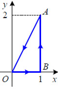
Area bounded by contour L let's denote D. If the functions P(x, y) , Q(x, y) and their partial derivatives and are functions continuous in the domain D, then to calculate the curvilinear integral you can use Green’s formula:

Thus, the calculation of a curvilinear integral over a closed contour is reduced to the calculation of a double integral over the area D.

Green's formula remains valid for any closed region, which can be drawn by drawing additional lines to a finite number of simple closed regions.

Example 1. Calculate line integral

,

If L- triangle outline OAB, Where ABOUT(0; 0) , A(1; 2) and B(1; 0) . The direction of traversing the circuit is counterclockwise. Solve the problem in two ways: a) calculate the curvilinear integrals on each side of the triangle and add the results; b) according to Green's formula.

a) Calculate the curvilinear integrals on each side of the triangle. Side O.B. is on the axis Ox, so its equation will be y= 0 . That's why dy= 0 and we can calculate the curvilinear integral along the side O.B. :

Side equation B.A. will x= 1 . That's why dx= 0 . We calculate the curvilinear integral along the side B.A. :

Side equation A.O. using the formula of the equation of a straight line passing through two points, let’s create:

.

Thus, dy = 2dx. We calculate the curvilinear integral along the side A.O. :

This curvilinear integral will be equal to the sum of the integrals along the edges of the triangle:

.

b) Let's apply Green's formula. Because , , That . We have everything we need to calculate this closed-loop integral using Green’s formula:

As you can see, we got the same result, but according to Green’s formula, calculating the integral over a closed loop is much faster.

Example 2.

,

Where L- contour OAB , O.B.- parabola arc y = x², from point ABOUT(0; 0) to point A(1; 1) , AB And B.O.- straight segments, B(0; 1) .

Solution. Since the functions are , , and their partial derivatives are , , D- area limited by contour L, we have everything to use Green’s formula and calculate this closed-loop integral:

Example 3. Using Green's formula, calculate the curvilinear integral

, If L- the contour formed by the line y = 2 − |x| and axis Oy .

Solution. Line y = 2 − |x| consists of two rays: y = 2 − x, If x≥ 0 and y = 2 + x, If x < 0 .

We have functions , and their partial derivatives and . We substitute everything into Green's formula and get the result.

These formulas connect the integral over a figure with some integral over the boundary of a given figure.

Let the functions be continuous in the domain DÌ Oxy and on its border G; region D– connected; G– piecewise smooth curve. Then true Green's formula:

here on the left is a curvilinear integral of the first kind, on the right is a double integral; circuit G goes counterclockwise.

Let T– piecewise smooth bounded two-sided surface with piecewise smooth boundary G. If the functions P(x,y,z), Q(x,y,z), R(x,y,z) and their first order partial derivatives are continuous at points of the surface T and borders G, then it occurs Stokes formula:

(2.23)

on the left is a curvilinear integral of the second kind; on the right – surface integral of the second kind, taken along that side of the surface T, which remains to the left when traversing the curve G.

If a connected region WÌ Oxyz limited by a piecewise smooth, closed surface T, and the functions P(x,y,z), Q(x,y,z), R(x,y,z) and their first order partial derivatives are continuous at points from W And T, then it occurs Ostrogradsky-Gauss formula:

(2.24)

on the left – surface integral of the second kind over the outer side of the surface T; on the right – triple integral over the area W.

Example 1. Calculate the work done by the force when traversing the point of its application of the circle G: , starting from the axis Ox, clockwise (Fig. 2.18).

Solution. Work is equal to . Let’s apply Green’s formula (2.22), placing the “-” sign on the right before the integral (since the circuit is traversed clockwise) and taking into account that P(x,y)=x-y, Q(x,y)=x+y. We have:
,
Where S D– area of ​​a circle D: , equal to . As a result: – the required work of force.

Example 2. Calculate integral , If G there is a circle in the plane z=2, going around counterclockwise.

Solution. Using the Stokes formula (2.23), we reduce the original integral to the surface integral over a circle T:
T:

So, given that , we have:

The last integral is a double integral over a circle DÌ Oxy, on which the circle was projected T; D: . Let's move on to polar coordinates: x=r cosj, y=r sinj, jÎ, r O. As a result:
.

Example 3. Find stream P T pyramids W: (Fig. 2.19) in the direction of the outer normal to the surface.

Solution. The flow is . Applying the Ostrogradsky-Gauss formula (2.24), we reduce the problem to calculating the triple integral over the figure W-pyramid:

Example 4. Find stream P vector field through the complete surface T pyramids W: ; (Fig. 2.20), in the direction of the outer normal to the surface.

Solution. Let us apply the Ostrogradsky-Gauss formula (2.24), where V– volume of the pyramid. Let's compare with the solution of direct calculation of the flow ( – faces of the pyramid).

,
since the projection of faces onto the plane Oxy has zero area (Fig. 2.21),